

Coupled Transmission Lines and Crosstalk
When two coplanar parallel traces run in close proximity over the coupled length, as shown in Figure 1, they are electromagnetically coupled together.
When two complimentary signals are transmitted, there is mutual electromagnetic coupling defined by amount of mutual inductance and capacitance. This is known as differential signaling. The differential impedance, (Zdiff), is the instantaneous impedance of a pair of transmission lines.
The impedance of each trace, when driven differentially, is known as the odd-mode impedance (Zodd). Conversely, when each trace is driven with the same polarity, the impedance of each trace is known as the even-mode impedance (Zev).
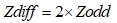
Differential impedance is simply twice the odd-mode impedance:
Equation 1
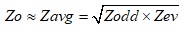
When Zodd = Zev, the traces are deemed to be uncoupled and there will be no crosstalk (XTalk). The characteristic impedance (Zo) of a single trace, in isolation, is equal to the geometric average (Zavg) of Zodd and Zev. When Zodd and Zev are not equal, there will be some level of XTalk, depending on the space between traces. In this case, Zo is approximately equal to Zav and is given as:
Equation 2
Crosstalk
There are two types of XTalk generated; Near-End (NEXT), or backwards XTalk, and Far-End (FEXT), or forward XTalk.
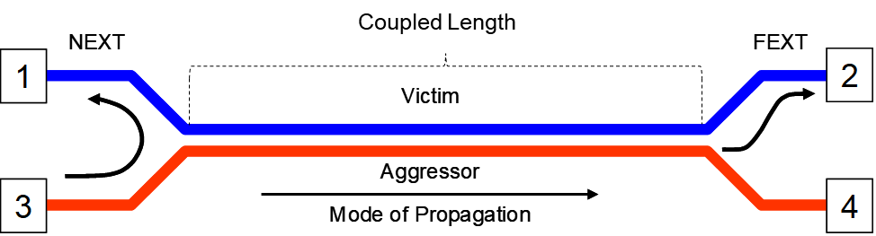
Figure 1. Illustration of NEXT and FEXT. As the aggressor signal propagates from port 3 to port 4, Near-End XTalk appears on port 1 and Far-End XTalk appears on port 2 after one time delay (TD) of the interconnect.
NEXT
Refer to Figure 1. Through electromagnetic coupling, NEXT voltage (Vb) is related to the coupled current through a terminating resistor (not shown) at port 1; when driven by an aggressor voltage (Va) at port 3. When port 1 is terminated, the backward XTalk coefficient (Kb) is defined by:
Equation 3

Where:
Vb = the voltage at port 1
Va = the peak voltage of the aggressor at port 3
The general signature of the NEXT waveform, for a gaussian step aggressor, is shown in Figure 2. Va is the aggressor voltage at port 3 of Figure 1. Vb is the NEXT voltage at port 1. The NEXT voltage continues to increase in response to the rising edge of the aggressor until it saturates after the aggressor’s rise-time. The green waveform (VaFE) is the aggressor voltage at port 4 after one time delay (TD). The duration of Vb waveform lasts for 2TD of the coupled length.
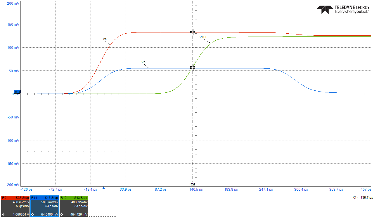
Figure 2. NEXT voltage signature, Vb in response to a gaussian step aggressor, Va. The duration of NEXT is equal to 2TD of the coupled length. VaFE is the aggressor voltage shown after one TD. simulated with Teledyne Lecroy WavePulser 40iX software.
When TD is equal to one-half of the linear risetime, the NEXT voltage becomes saturated. The minimum length to reach saturation is known as the saturated length (Lsat), and is given by [1]:
Equation 4
Where:
Lsat = the saturation length for near-end cross talk in inches
RT = linear risetime to reach Va in ns
c = the speed of light = 11.8 in nsec
Dkeff = the effective dielectric constant surrounding the trace.
For example, a signal with a linear RT of 0.1 nsec, to reach an aggressor voltage of 1V using FR4 material, with a Dkeff of 4, the saturation length in stripline is:
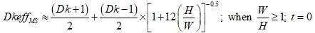
Important note: In PCB stripline construction, Dkeff is the Dk of the dielectric mixture of core and prepreg. But in microstrip, without solder mask, Dkeff is the mixture of Dk of air and Dk of the substrate. It is very difficult to predict the exact Dkeff in microstrip without a field solver, but a good approximation can be obtained by [3]:
Equation 5
Where:
DkeffMS = effective dielectric constant surrounding the trace in microstrip
Dk = dielectric constant of the material
H = height of dielectric
W = trace width
t = trace thickness
For example, a signal with a linear RT of 0.1 ns, to reach an aggressor voltage of 1V and DkeffMS of 2.64, the saturation length in microstrip is:
If the coupled length (Lcoupled) is less than Lsat, the NEXT voltage will peak at a value less than the saturated NEXT voltage. The actual NEXT voltage, Vb, is scaled by the ratio of coupled length to saturation length and is given by [1]:
Equation 6
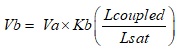
For example, for a coupled of length of 100 mils and saturated length of 295 mils, NEXT voltage will be (100/295) or 33.9% of the saturated NEXT voltage.
NEXT vs Coupled Length in Stripline
Figure 3 plots NEXT voltage vs coupled lengths for 100 mils, 295 mils and 590 mils representing less than, equal to and greater than Lsat respectively. For a coupled stripline geometry modeled with Polar SI9000 field solver (Figure 3B) Kb is 0.065.
Each length was simulated in Polar Si9000 and touchstone files were imported into Keysight PathWave ADS software for further analysis. The results are plotted in Figure 3A.
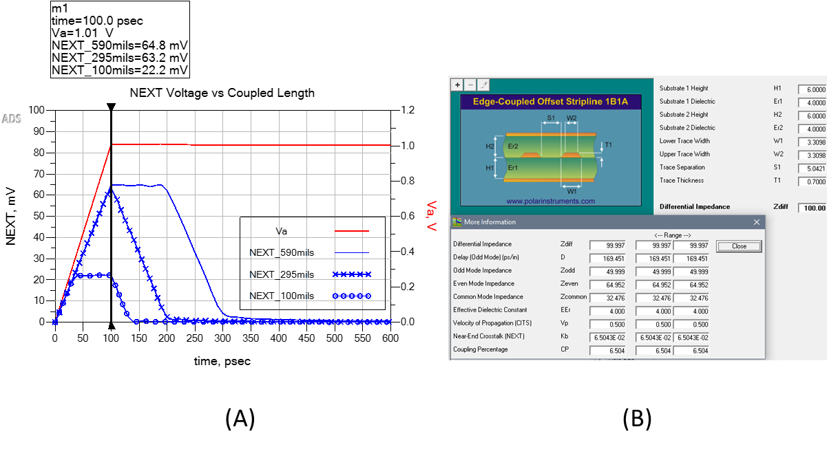
Figure 3. Example of NEXT voltage vs couple lengths of 100 mils, 295 mils and 590 mils in stripline. Modeled with Polar Si9000 and simulated with Keysight PathWave ADS.
As can be seen, using a 1V aggressor with a linear risetime of 0.1 ns and a saturated length of 295 mils, the NEXT voltage is 63.2 mV, compared to full saturated NEXT voltage of 64.8 mV. With a coupled length of 100 mils, NEXT voltage saturates at 22.2 mV, for the duration of the aggressor’s risetime, compared to 22.03 mV predicted by Equation 6 [1].
NEXT vs Coupled Length in Microstrip
Each length was then simulated in Polar Si9000 and touchstone files were imported into Keysight PathWave ADS software for further analysis. The results are plotted in Figure 4A.

Figure 4. Example of NEXT voltage vs couple lengths of 100 mils, 363 mils and 590 mils in microstrip. Modeled with Polar Si9000 and simulated with Keysight PathWave ADS.
As can be seen, using a 1V aggressor with a linear risetime of 0.1 ns and a saturated length of 363 mils, the NEXT voltage is 54.6 mV, compared to full saturated NEXT voltage of 54.9 mV. With a coupled length of 100 mils, NEXT voltage saturates at 15.8 mV for the duration of the aggressor’s risetime, compared to 15.1 mV predicted by Equation 6.
The magnitude of the NEXT voltage is a function of the coupled spacing between the two traces. As the two traces are brought closer together, the mutual capacitance and inductance increases and thus the NEXT voltage, Vb, will increase as defined by [1]:
Equation 7

Where:
Kb = backward XTalk (NEXT) coefficient
Va = aggressor voltage
Cm = mutual capacitance per unit length
Lm = mutual inductance per unit length
Co = trace capacitance per unit length
Lo = trace inductance per unit length
Unfortunately, the only practical way to calculate Kb is to use a 2D field solver to get the inductive and capacitance matrix elements from a field solver.
Alternatively, if only the odd and even mode impedances are known, then Kb is given as [2]:
Equation 8

Where:
Zterm = victim input termination impedance, normally the characteristic impedance (Zo) of a single trace.
When, Zterm is open circuit, Kb’ is given as [2]:
Equation 9

FEXT
FEXT voltage is correlated to the coupled current through a terminating resistor (not shown) at port 2 of Figure 1. The forward XTalk coefficient, Kf, is equal to the ratio of FEXT voltage to aggressor voltage at the far end, defined as:
Equation 10

Where:
Vf = the far end XTalk voltage
VaFE = the peak voltage of the aggressor at far-end
The general signature of the FEXT waveform, for a gaussian step aggressor, is shown in Figure 5. Vf is the forward XTalk voltage at port 2 of Figure 1. VaFE is the aggressor voltage appearing at the far end port 4. FEXT voltage differs from NEXT in that it only appears as a pulse at TD after the signal is launched. In this example, the negative going FEXT pulse is the derivative of the aggressor’s rising edge at TD. The opposite is true on the falling edge of an aggressor.

Figure 5. FEXT voltage signature, Vf, is forward XTalk (FEXT) voltage in response to a gaussian step aggressor voltage, VaFE. Simulated with Teledyne Lecroy WavePulser 40iX software.
Unlike the NEXT voltage, the peak value of FEXT voltage scales with the coupled length. It peaks when its amplitude grows to a level comparable to the voltage at 50% of the aggressor’s risetime at TD as shown in Figure 6. In this example, the coupled lengths are: 2, 4, 6, 8 and 10 inches respectively.
As the wave propagates along the transmission line, the RT degrades due to the dielectric dispersive loss. In the same way the aggressor waveform couples FEXT voltage onto the victim, FEXT voltage also couples noise back onto the aggressor affecting the risetime as shown. Due to superposition, the aggressor waveform shown at each TD is the sum of the FEXT voltage and the original transmitted waveform that would have appeared at TD with no coupling.

Figure 6. Microstrip FEXT voltage increase vs TD for coupled lengths of 2, 4, 6, 8 and 10 inches respectively. Simulated with Teledyne Lecroy WavePulser 40iX software.
If the rise-time at TD is known, the FEXT voltage can be predicted by [1];
Equation 11

Where:
Vf = FEXT voltage
VaFE = Far-end aggressor voltage
Kf = FEXT coefficient
Cm = Mutual capacitance per unit length
Lm = Mutual inductance per unit length
Co = Trace capacitance per unit
Lo = Trace inductance per unit length
RT = Risetime of aggressor signal at TD in sec
c = Speed of light
Dkeff = Effective dielectric constant surrounding the trace
Len = Length of trace
Although the inductive and capacitive matrix elements can be obtained using a 2D field solver, the rise-time is more difficult to predict because of risetime degradation, as well as impedance variations along the line causing reflections. But worst of all, as seen in Figure 6, is the forward XTalk coupling affecting the aggressor’s risetime makes it next to impossible to predict.
The only practical way to calculate Kf is to model and simulate the topology using a circuit simulator that supports coupled transmission lines. The circuit simulator should have an integrated 2D field solver built in to allow automatic generation of a coupled transmission line model from the cross-sectional information.
Since the dielectric surrounding the traces in stripline is more homogeneous, than it is in microstrip, the best way to significantly reduce, or eliminate FEXT, is to route the traces in stripline geometry. Depending on the difference in Dk between core and prepreg used in the stackup, there is always a probability there will be some small amount of FEXT generated. The best way to mitigate this is to choose cores and prepregs to have similar values of Dk when designing the stackup.
References:
- E. Bogatin, “Signal Integrity Simplified”, 2nd edition, Prentice Hall PTR, 2010
- B. Young, "Digital Signal Integrity", Upper Saddle River, NJ: Prentice Hall, 2001
- E. O. Hammerstad, "Equations for Microstrip Circuit Design," 1975 5th European Microwave Conference, 1975, pp. 268-272, doi: 10.1109/EUMA.1975.332206.
- E. Bogatin, B. Simonovich, “Dramatic Noise Reduction using Guard Traces with Optimized Shorting Vias”, DesignCon 2013, Santa Clara, CA, USA
